import pandas as pd
import numpy as np
from sklearn.model_selection import train_test_split

# Importing eshop_revenues
eshop_revenues = pd.read_csv("https://raw.githubusercontent.com/Datakortex/Datasets/refs/heads/main/eshop_revenues.csv")Model Validation and Performance Evaluation
Introduction
Up to now, we have trained models on a single training set and evaluated their performance on a separate test set. We used metrics such as MAE for regression and accuracy for classification to assess how well the models performed on unseen data. In earlier chapters, we also experimented with adjusting models and comparing alternatives, including hyperparameter changes, to improve performance. However, this approach is not ideal, since repeatedly using the test set for model selection effectively turns it into part of the training process. This leads to overly optimistic performance estimates and undermines its role as a final, unbiased evaluation tool.
In this chapter, we focus on validating and measuring model performance in a more principled way. We introduce resampling methods that allow us to evaluate models more reliably and systematically by repeatedly splitting the data into training and evaluation subsets. We also discuss how performance metrics should be chosen based on the goal of the analysis, since different metrics can lead to different conclusions about which model performs best.
Performance Evaluation
In the previous chapters, we highlighted that the training set should not be used to evaluate the predictive performance of a model, due to the risk of overfitting. Unless the model is very simple, such as a linear regression with only a few predictors, most models will tend to overfit the dataset on which they are trained. For this reason, we introduced the holdout method, where a subset of the data—called the test set—is kept aside to test model performance.
However, we also followed this approach mainly for simplicity. In practice, we emphasized that using the test set as a guide to tweak or improve our models makes it effectively part of the training process. This should never be the case. As Trevor Hastie, a well-known expert in machine learning, states, “ideally the test set should be kept in a vault, and be brought out only at the end of the data analysis” (Hastie et al., 2009; Lantz, 2023).
Validation Set
The simplest way to avoid using the test set during model selection is to introduce an additional subset of the original dataset. This dataset is usually called the validation set, and it is kept separate from the test set. The idea is straightforward: we train different models on the training set, evaluate their performance on the validation set, and then select the model that performs best. After identifying a satisfactory model, we evaluate it one final time on the test set to obtain an unbiased estimate of its performance.
However, even when using a validation set, the same issue can arise. A model may eventually overfit the validation set, meaning that it performs well on validation data but does not generalize well to truly unseen data. For this reason, we often rely on resampling methods, especially when the dataset is large enough to support them. Resampling methods create multiple training and testing splits from the same dataset. Instead of relying on a single split, we repeat the evaluation process several times, leading to more reliable estimates of model performance.
K-fold Cross Validation
One of the most commonly used resampling techniques is k-fold cross-validation. The idea is simple: we start by splitting the training dataset into \(k\) equally sized parts, called folds. For example, if \(k = 5\), the data is divided into five folds. In each iteration, the model is trained on \(k - 1\) folds (the analysis set) and evaluated on the remaining fold (the assessment set). This process is repeated \(k\) times so that each fold serves exactly once as the assessment set.
As a result, we obtain \(k\) performance values, one from each fold. Since each value comes from a different assessment set, the result is not a single estimate but a distribution of performance values. For example, if we use MAE as the evaluation metric, we obtain \(k\) different MAE values. Instead of summarizing performance with a single number, we can describe this distribution using the mean and standard deviation, which gives us both an estimate of expected performance and information about its variability. Importantly, every observation in the training set is used exactly once for assessment and multiple times in the analysis sets, ensuring that all data points contribute to both model fitting and evaluation.
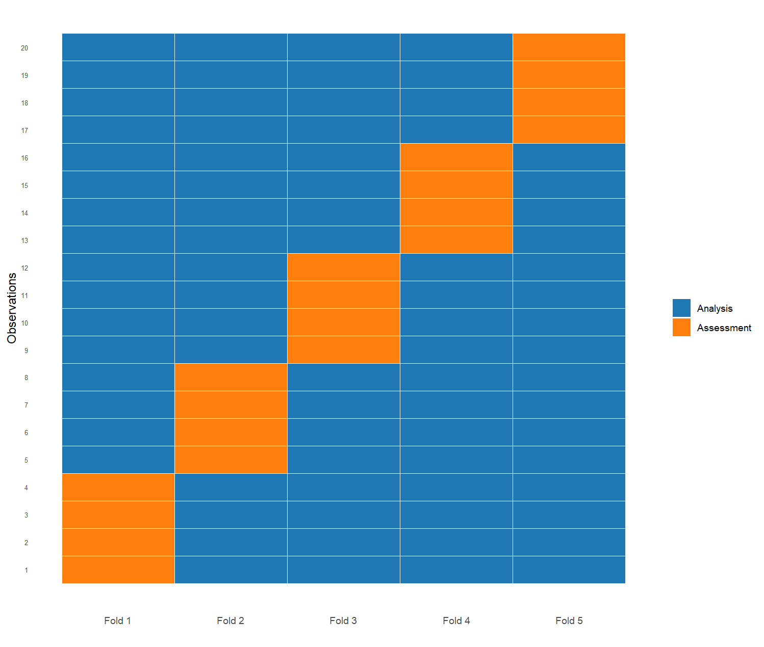
In the plot above, the first fold assigns the first 4 observations to the assessment (test) set, with the remaining 16 observations used for analysis (training). In the second fold, the next group of 4 observations forms the assessment set, while all other observations are used for analysis. This procedure is repeated until each observation has been used exactly once in the assessment set across the five folds, with the remaining observations forming the corresponding training sets.
Nothing prevents us from increasing the number of folds. Common choices are 5-fold or 10-fold cross-validation. In general, a larger number of folds leads to a more detailed evaluation, but also increases computational cost.
Even though k-fold cross-validation produces multiple performance estimates that resemble a distribution, it is worth noting that these observations are not independent. The method relies on repeated reuse of the same data points across different analysis sets, which introduces dependence between the folds. As a result, the performance values obtained from each fold are correlated, since the analysis sets overlap significantly.
This means that cross-validation does not generate independent samples of model performance in a strict statistical sense. Instead, it provides a practical and highly useful approximation of model generalization performance. For this reason, cross-validation should be interpreted as an estimation tool rather than a formal inferential procedure.
Repeated K-fold Cross Validation
One potential drawback of standard k-fold cross-validation is that the results can still vary depending on how the data is split (Kuhn & Johnson, 2019). To reduce this variability, we can use repeated k-fold cross-validation. In this approach, the entire cross-validation procedure is repeated multiple times using different random partitions of the training data. This produces a larger set of performance estimates, leading to a more stable and reliable evaluation of model performance (Kuhn et al., 2022). Averaging across repeats reduces sensitivity to any single data split and improves the robustness of both the expected performance estimate and its variability.
The main drawbacks of this method are that it is computationally more expensive than standard k-fold cross-validation, since the full resampling procedure is repeated multiple times. Additionally, it does not resolve the underlying dependence between resamples. The assessment sets are still derived from overlapping training data, so the assumption of independent sampling remains violated (Lantz, 2023).
Leave-One-Out Cross-Validation (LOOCV)
A special case of k-fold cross-validation is leave-one-out cross-validation (LOOCV). In this approach, the number of folds is equal to the number of observations in the dataset. This means that in each iteration, we use all observations except one for training, and we evaluate the model on the single remaining observation.
This process is repeated for every observation in the dataset. As a result, we obtain as many performance values as there are observations. These values can again be summarized using the mean and standard deviation to estimate model performance.
LOOCV can be seen as the most extreme form of cross-validation, since it maximizes the amount of training data used in each iteration. In each step, the model is trained on almost the entire dataset, which can lead to very low bias in the performance estimate. However, this comes at a cost. Because each validation set contains only one observation, the resulting performance estimates can have high variance, especially if the dataset contains noise or outliers.
From a practical perspective, LOOCV is computationally expensive, since the model must be fitted as many times as there are observations. For large datasets, this quickly becomes infeasible, which is why LOOCV is rarely used in practice when k-fold cross-validation provides a reasonable alternative.
Monte Carlo Cross Validation
Another important resampling method is Monte Carlo cross-validation, also known as random subsampling. In this approach, we repeatedly generate random splits of the training dataset into analysis and assessment sets (for example, 80% analysis and 20% assessment). Unlike k-fold cross-validation, these splits are not mutually exclusive. This means that the same observation can appear multiple times in different assessment sets, or may not appear at all in some iterations, something that is illustrated in the plot below:
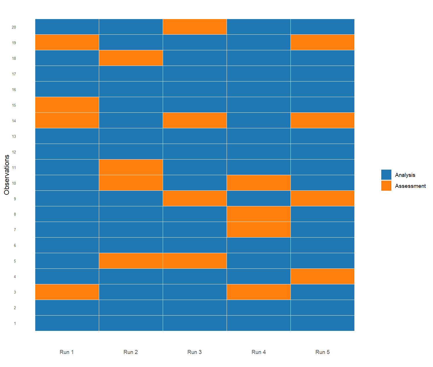
Due to overlapping splits, Monte Carlo cross-validation behaves differently from k-fold cross-validation. It provides more flexibility in how the data is split, but it does not guarantee that all observations are used equally often in validation. In return, it is useful when we want direct control over the size of the analysis and assessment sets without requiring strict partitioning structure. A typical example is evaluating a house price prediction model by repeatedly creating random 80/20 splits of the data to assess performance. In this case, we are more interested in how the model performs under different realistic samples of the data rather than ensuring that every observation is used equally often in validation, since each large split is already reasonably representative of the problem.
Due of this structural difference, Monte Carlo cross-validation and k-fold cross-validation also differ in terms of the bias–variance trade-off. In this context, bias refers to systematic error in the estimated model performance compared to the true generalization performance, while variance refers to how much the performance estimates fluctuate across different resamples.
K-fold cross-validation tends to produce lower variance estimates because every observation is used in a more structured and balanced way across folds. However, it may introduce slightly higher bias depending on the choice of K, since each model is trained on a fixed and somewhat constrained proportion of the data in every iteration. Monte Carlo cross-validation, on the other hand, can reduce bias because the random splits allow more flexibility in how training and validation sets are formed, and each split more closely resembles an independent holdout experiment. However, this comes at the cost of higher variance, since results depend more strongly on the randomness of the splits and the uneven participation of observations across iterations.
In short, Monte Carlo cross-validation tends to provide a more accurate estimate of the true generalization performance but with higher uncertainty (variance), whereas k-fold cross-validation produces more stable (lower variance) but slightly more constrained and potentially more biased estimates.
Bootstrap Resampling
In Chapter Tree-Based Models, we used bootstrap resampling for bagged trees and random forests to generate different decision trees. This same resampling technique can also be used to evaluate model performance. As discussed in that chapter, bootstrap works by repeatedly drawing samples with replacement from the original training dataset. This means that some observations may appear multiple times in a given resample, while others may not appear at all.
Each bootstrap sample is used to fit a model, and performance is evaluated on the observations that were not included in that sample. These are known as the out-of-bag (OOB) observations. By repeating this process many times, we obtain a distribution of performance estimates, similar in spirit to cross-validation.
The key difference between bootstrap and cross-validation lies in how the resamples are constructed. In k-fold and Monte Carlo cross-validation, the data is partitioned into analysis and assessment sets without replacement. In bootstrap, however, sampling is performed with replacement, which allows the same observation to be selected multiple times within a single resample.
Because of this, bootstrap samples have a different structure from the original dataset. On average, each bootstrap sample contains about 63% unique observations, while the remaining observations are left out and used for evaluation as OOB samples. This proportion arises from the sampling-with-replacement mechanism and converges to approximately 0.632 as the dataset size increases, a result that can be justified using large-sample (Law of Large Numbers) arguments. This property makes bootstrap particularly useful when the dataset is small, since it allows us to generate many alternative training sets without requiring additional data.
In terms of bias and variance, bootstrap methods often produce relatively low-bias estimates of model performance, but they can exhibit higher variance depending on the model and dataset size. This is partly because each bootstrap sample is effectively trained on approximately 63% unique observations, which introduces additional variability across resamples. However, the main strength of bootstrap lies not in point estimation alone, but in quantifying uncertainty, making it especially useful when the goal is not only to compare models but also to assess the stability of predictions.
In practice, bootstrap resampling is widely used for estimating confidence intervals, assessing model stability, and quantifying the variability of model performance. Unlike cross-validation methods, which mainly focus on estimating predictive performance, bootstrap is particularly useful when the goal is to understand how much the results would change under different samples of the data. For this reason, it is a key tool in data science, especially when data is limited or when quantifying uncertainty is an important part of the analysis.
Rolling Origin Forecasting
All the methods discussed up to now—k-fold cross-validation, Monte Carlo cross-validation, and bootstrap—assume that there is no time component in the data. In other words, they assume that observations are independent and do not follow a specific order. In practice, however, this assumption is often violated. Many datasets have a clear temporal structure, where the order of observations is essential.
A classic example is ice cream sales, where demand increases during summer and decreases during winter due to seasonality. In this case, randomly shuffling the data would break the temporal structure of the seasonal pattern and lead to unrealistic evaluation results.
For this reason, it does not make sense to fit a model on future observations and then evaluate it on past ones. In practice, models should always be trained on past data and evaluated on future data, since this reflects the real-world forecasting setting.
When there is a clear ordering in the data, it is therefore recommended to use rolling origin forecasting resampling methods (Hyndman & Athanasopoulos, 2021). In rolling origin forecasting, the idea is to respect the temporal order of the data when creating training and test sets.
Instead of randomly splitting the data, we use either an expanding window or a sliding window approach. In an expanding window, the analysis set starts with an initial segment of the data and grows over time, meaning that all past observations are retained as new data becomes available. In a sliding window, by contrast, the analysis set has a fixed size, and as we move forward in time, older observations are removed while newer ones are added. This allows the model to focus only on the most recent data, which can be useful when older patterns become less relevant. Both approaches create splits that reflects how the model would actually be used in practice: learning from the past and predicting the future.
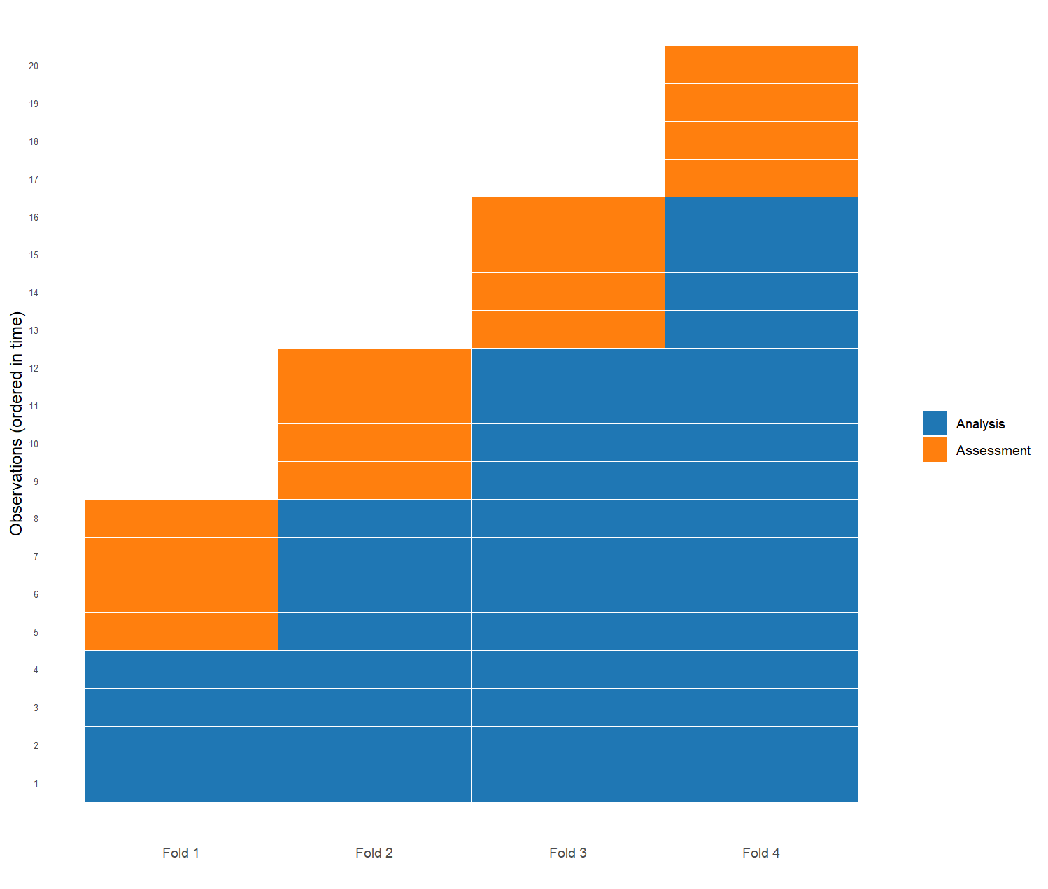
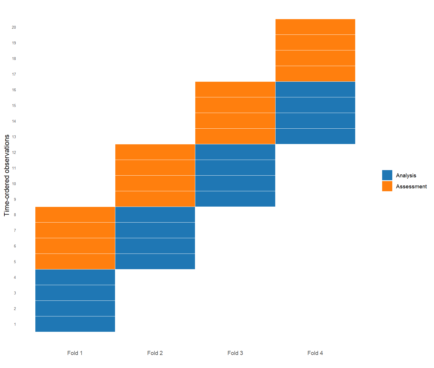
It is worth noting that the important element here is not strictly time itself, but the order of the observations. What matters is that the distribution of the variables may change as we move forward, a concept known as data drift. For example, customer behavior in an online store may evolve due to seasonality, marketing campaigns, or changes in preferences. Similarly, financial markets may behave differently during periods of crisis compared to stable periods.
This phenomenon is closely related to a key challenge in machine learning known as model drift. Model drift occurs when a model that performs well on recent historical data gradually becomes less accurate over time, even though it was trained on relatively recent observations. This happens because the relationship between predictors and the outcome changes, meaning that the assumptions of the model are no longer valid.
In practice, this is one of the main challenges in time-dependent data. A model that performs very well today may start to degrade tomorrow, not because it is incorrectly specified, but because the environment has changed. Rolling origin forecasting helps us evaluate models in a way that respects this evolving structure and provides a more realistic estimate of future performance.
Choosing the Appropriate Resampling Method
All the discussed resampling methods have the same goal: to produce performance estimates that generalize to previously unseen data. The next question is which method is most appropriate in each case. As always, the answer is that it depends on the problem and the data. For this reason, we need to consider how the model will be used in practice and whether there is a meaningful structure or ordering in the data.
Most of the time, our goal is to train a model using data available today to make predictions about the future. In these cases, we must respect the temporal structure of the data, and rolling origin forecasting is often the most appropriate choice, since it mimics how the model will actually be deployed in practice.
When there is no clear ordering in the data, and there is no strong evidence of model drift or distribution shift, k-fold cross-validation or repeated k-fold cross-validation are solid and widely used choices due to their balance between stability and computational efficiency, assuming a large enough dataset.
Monte Carlo cross-validation can be useful when we want more flexibility in how training and assessment sets are constructed, or when we are interested in assessing performance under many different random holdout scenarios. Bootstrap, on the other hand, is particularly appropriate when the main goal is not only prediction but also statistical inference, such as estimating confidence intervals or quantifying uncertainty in model performance.
It is important to emphasize that all these resampling methods are applied within the training set. Best practice is to always keep a final test set separated in a “vault” that is only used once, after model selection and tuning are complete. This test set provides an unbiased estimate of final model performance. A separate test set may be omitted only in cases where the dataset is extremely small and alternative validation strategies are necessary (Kuhn et al., 2022).
Finally, once a model has been selected and validated, the most common practice is to refit it on all available training data—combining the original training, validation, and resampling information where appropriate—so that the final model benefits from the maximum amount of information before being used for future predictions (Lantz, 2023).
Performance Evaluation with Scikit-learn
Now that we have discussed different resampling methods, we will use scikit-learn to apply them in practice. For simplicity, we will use linear regression on the dataset eshop_revenues. Let’s start by importing the dataset:
To create an additional validation set apart from the test set, we split the data in two steps using train_test_split(). We first set aside 20% as the test set, and then split the remaining 80% so that the validation set ends up being another 20% of the original data (25% of the remaining 80%), leaving 60% for training:
# Setting aside the test set
train_val, test_set = train_test_split(
  eshop_revenues,
  test_size = 0.2,
  random_state = 123
  )

# Splitting the remainder into training and validation sets
training_set, validation_set = train_test_split(
  train_val,
  test_size = 0.25,
  random_state = 123
  )

# Printing the resulting shapes
training_set.shape, validation_set.shape, test_set.shape
((78, 7), (26, 7), (26, 7))The resulting split now contains three parts: a training set, a validation set, and a test set, with 78, 26, and 26 observations respectively. Next, we separate the predictors from the target variable, Revenue, for the training and validation sets:
# Separating predictors and target
X_train = training_set.drop(columns = "Revenue")
y_train = training_set["Revenue"]

X_val = validation_set.drop(columns = "Revenue")
y_val = validation_set["Revenue"]
We can now fit a linear regression model on the training set and evaluate performance on the validation set. We use all available predictors, with Revenue as the target variable:
from sklearn.linear_model import LinearRegression

# Fitting linear regression model using all predictors
lm_fit = LinearRegression()
lm_fit.fit(X_train, y_train)
As in previous chapters, we generate predictions and compute the MAE. This time, however, we evaluate performance on the validation set rather than the test set:
# Making predictions on the validation set
predictions = lm_fit.predict(X_val)

# Calculating MAE
np.mean(np.abs(y_val - predictions))np.float64(8354.08528800624)On average, the predicted revenues differ from the actual revenues by approximately €8,354.
We repeat the process using a more complex model that includes all available interactions between predictors. Since this means applying a transformation step (creating the interactions) before fitting the model, this is a good moment to introduce a pipeline. A pipeline simply chains together a sequence of steps—typically one or more preprocessing transformations followed by a model—into a single object. Instead of manually transforming X_train, then X_val, then any future dataset the same way before fitting or predicting, we define the steps once and the pipeline applies them consistently every time we call fit() or predict(). This becomes especially valuable with resampling later in the chapter, where the same transformation needs to be reapplied correctly across many different training splits.
A pipeline is built by passing a list of (name, step) pairs, where each name is just a label we choose and step is the actual transformer or model.A pipeline is built by passing a list of (name, step) pairs, where each name is just a label we choose and step is the actual transformer or model. We import Pipeline from sklearn.pipeline. Here, we use PolynomialFeatures with degree = 2 and interaction_only = True, which generates the original predictors together with all pairwise interactions between them, but no squared terms:
from sklearn.preprocessing import PolynomialFeatures
from sklearn.pipeline import Pipeline

# Building a pipeline with interactions and the linear model
lm_pipeline = Pipeline([
  ("interactions", PolynomialFeatures(degree = 2,
                                      interaction_only = True,
                                      include_bias = False)),
  ("lm", LinearRegression())
  ])

# Fitting linear regression model using all predictors and their interactions
lm_pipeline.fit(X_train, y_train)

# Making predictions on the validation set
predictions_with_interactions = lm_pipeline.predict(X_val)

# Calculating MAE
np.mean(np.abs(y_val - predictions_with_interactions))np.float64(6864.6889786953125)When we call lm_pipeline.fit(X_train, y_train), the pipeline first applies PolynomialFeatures to X_train to create the interaction terms, then fits the LinearRegression model on that expanded set of predictors. When we later call lm_pipeline.predict(X_val), it automatically applies the same PolynomialFeatures transformation to X_val before generating predictions—we never have to remember to do that step ourselves.
In our case, the MAE decreases substantially, suggesting that the more complex model provides better predictive performance on the validation set. Based on this result, we select this model as the final candidate, which we refit on the training and validation sets and evaluate it on the test set:
# Combining training and validation sets into a single dataframe
training_validation_set = pd.concat([training_set, validation_set], ignore_index = True)

X_train_val = training_validation_set.drop(columns = "Revenue")
y_train_val = training_validation_set["Revenue"]

X_test = test_set.drop(columns="Revenue")
y_test = test_set["Revenue"]

# Refitting linear regression model
lm_pipeline.fit(X_train_val, y_train_val)

# Making predictions on the test set
predictions_with_interactions = lm_pipeline.predict(X_test)

# Calculating MAE
np.mean(np.abs(y_test - predictions_with_interactions))np.float64(4909.987100395843)The MAE on the test set is significantly lower than on the validation set, something that can occur when the dataset is small. This large difference illustrates an important point: performance estimates depend on the specific split of the data. For this reason, relying on a single validation split can be unstable, and motivates the use of resampling methods discussed in the previous section.
Overall, this example shows how a simple validation approach mirrors the traditional train-test procedure, while also highlighting its limitations in terms of variability and reliability.
To use resampling methods, we rebuild the same pipeline—preprocessing and model combined into a single object—and reuse it across every resampling scheme discussed in this chapter:
# Rebuilding the pipeline with interactions and the linear model
lm_workflow = Pipeline([
  ("interactions", PolynomialFeatures(degree = 2,
                                      interaction_only = True,
                                      include_bias = False)),
  ("lm", LinearRegression())
  ])
Before we can apply resampling, we also need to define the resampling scheme itself. We use RepeatedKFold to generate the analysis/assessment splits, with n_splits = 10 and n_repeats = 3, corresponding to 3 repetitions of 10-fold cross-validation. Calling split(X_train) on it and wrapping the result in list() gives us the actual (train_idx, test_idx) pairs:
from sklearn.model_selection import RepeatedKFold

# 10x3 (repeated) cross-validation folds
folds_rep_cv = RepeatedKFold(
  n_splits = 10,
  n_repeats = 3,
  random_state = 123)
splits_rep_cv = list(folds_rep_cv.split(X_train))

# Printing the first few splits
splits_rep_cv[0:2]
[(array([0, 1, 2, 3, 5, 6, 7, 8, 9, 10, 11, 12, 13, 14, 15, 16,
17, 18, 19, 20, 21, 22, 24, 25, 26, 27, 28, 30, 31, 32,
33, 34, 35, 36, 37, 38, 39, 40, 41, 42, 43, 44, 45, 46,
47, 48, 49, 50, 51, 52, 54, 55, 56, 57, 58, 59, 62, 63,
65, 66, 67, 68, 69, 71, 72, 73, 74, 75, 76, 77]),
array([4, 23, 29, 53, 60, 61, 64, 70])),
(array([0, 1, 2, 3, 4, 5, 6, 7, 10, 11, 12, 13, 14, 15, 16, 17,
18, 19, 20, 21, 22, 23, 25, 26, 27, 28, 29, 30, 31, 32,
33, 34, 35, 36, 37, 38, 39, 40, 41, 42, 43, 45, 46, 47,
48, 49, 50, 51, 52, 53, 54, 55, 56, 57, 58, 59, 60, 61,
62, 64, 65, 66, 67, 68, 69, 70, 71, 72, 73, 74]),
array([8, 9, 24, 44, 63, 75, 76, 77]))]The object splits_rep_cv is a list with 30 elements—one per resample (10 folds × 3 repeats). Each element is itself a tuple of two NumPy arrays: the first holds the row positions used for the analysis (training) set, and the second holds the row positions used for the assessment (test) set. These are positions within X_train (0-based, like Python indexing in general), not the original DataFrame index values, which is why we index into X_train with .iloc[] rather than .loc[] whenever we use them later in this chapter.
Now our pipeline is ready, and we can apply resampling methods to evaluate it. We use the function cross_validate() from scikit-learn, which fits the pipeline on each analysis set and evaluates it on the corresponding assessment set, returning a dictionary of per-resample scores. It accepts a scoring argument to specify the metric, and a cv argument that takes any cross-validation splitter—or, just as easily, a plain list of (train_idx, test_idx) tuples, which is what lets us reuse it later for Monte Carlo and bootstrap resampling without writing anything custom.
Note that scikit-learn always treats a higher score as better. Since a lower MAE is actually better, scikit-learn flips its sign internally—that’s why the metric is called "neg_mean_absolute_error" and why the values come back negative. We just negate them again to get the MAE back on its normal scale:
from sklearn.model_selection import cross_validate

# Fitting resamples
results_rep_cv = cross_validate(
  lm_workflow,
  X_train,
  y_train,
  cv = splits_rep_cv,
  scoring = "neg_mean_absolute_error"
  )

# Collecting results
mae_rep_cv = -results_rep_cv["test_score"]

# Printing the first few values
mae_rep_cv[0:5]
array([3118.28069634, 4847.07221651, 4308.2752312 ,
5999.9102573 , 7445.46998813])The object mae_rep_cv is a NumPy array with 30 values—one MAE per resample, in the same order as splits_rep_cv.
To summarize these into a mean and standard error, we use the following code:
# Summarizing mean and standard error across resamples
mae_rep_cv.mean(), mae_rep_cv.std(ddof = 1) / np.sqrt(len(mae_rep_cv))
(np.float64(5341.888190096755), np.float64(295.7540135937558))The output shows the average MAE across the 30 resamples, as well as the variability of this estimate across different splits of the training data. This provides a more robust estimate of model performance than a single train–validation split, since it reduces the dependence on one particular partition of the data.
If we also want the out-of-sample predictions for each resample—not just the aggregated score—cross_val_predict() covers the single-pass case (e.g. plain KFold), but it raises an error on RepeatedKFold, since each observation then belongs to more than one assessment set and the function expects a clean one-to-one partition. For repeated CV specifically, a short loop over the same splits gets us there instead:
from sklearn.base import clone

# Collecting out-of-sample predictions across all repeats
pred_rows = []
for i, (train_idx, test_idx) in enumerate(splits_rep_cv, start = 1):
  model = clone(lm_workflow)
  model.fit(X_train.iloc[train_idx], y_train.iloc[train_idx])
  preds = model.predict(X_train.iloc[test_idx])
  pred_rows.append(pd.DataFrame({
    "resample": i,
    "row": X_train.iloc[test_idx].index,
    "truth": y_train.iloc[test_idx].values,
    "prediction": preds
    }))

# Combining predictions from all resamples into a single dataframe
predictions_rep_cv = pd.concat(pred_rows, ignore_index = True)

# Printing the first few rows
predictions_rep_cv.head()| resample | row | truth | prediction | |
|---|---|---|---|---|
| 0 | 1 | 80 | 3343.82 | 6177.53 |
| 1 | 1 | 36 | 22791.06 | 22644.42 |
| 2 | 1 | 70 | 663.75 | 6217.12 |
| 3 | 1 | 106 | 2927.42 | -221.11 |
| 4 | 1 | 61 | 1426.59 | -221.87 |
Walking Through the Loop
This loop rebuilds, by hand, the out-of-sample predictions that
cross_validate()doesn’t give us directly. We start with an empty list, pred_rows, to collect one small DataFrame per resample, then loop over the 30 (train_idx,test_idx) pairs insplits_rep_cv, usingenumerate(..., start = 1)to also track a resample numberifrom1to30. For each resample,clone(lm_workflow)creates a fresh, unfitted copy of the pipeline—so each split gets its own independent model rather than repeatedly refitting (and overwriting) the same object—which we then fit on the analysis rows (train_idx) and use to predict on the held-out assessment rows (test_idx). Each iteration’s results are packaged into a small DataFrame recording which resample it came from, the original row index, the true value, and the predicted value, which gets appended topred_rows. Once the loop finishes,pd.concat(pred_rows, ignore_index = True)stacks all 30 of these small DataFrames into one long DataFrame,predictions_rep_cv, with one row per (resample, observation) pair across every resample.
For Monte Carlo cross-validation, we use the class ShuffleSplit() to generate the resamples, and pass it straight to cross_validate() exactly as before—only the cv argument changes:
from sklearn.model_selection import ShuffleSplit

# Monte Carlo cross-validation folds
folds_mc = ShuffleSplit(n_splits = 30,
                        train_size = 0.75,
                        random_state = 123)

# Fitting resamples
results_mc = cross_validate(lm_workflow,
                            X_train,
                            y_train,
                            cv = folds_mc,
                            scoring = "neg_mean_absolute_error")

# Flipping the sign to get MAE back on its normal scale
mae_mc = -results_mc["test_score"]

# Collecting results
mae_mc.mean(), mae_mc.std(ddof = 1) / np.sqrt(len(mae_mc))
(np.float64(5540.062634500627), np.float64(209.54553781355372))Next, we move to bootstrap resampling. Scikit-learn doesn’t ship a bootstrap splitter, so this is the one place we build the splits ourselves, using resample() from sklearn.utils to draw the in-bag sample and treating everything left out as the out-of-bag (OOB) assessment set. Once we have the list of (train_idx, test_idx) pairs, though, it plugs into cross_validate() the same way the other two did:
from sklearn.utils import resample

# Generates bootstrap splits: in-bag indices for training, OOB indices for evaluation
def bootstrap_splits(n_obs, n_times = 30, random_state = 123):
  rng = np.random.RandomState(random_state)
  indices = np.arange(n_obs)
  splits = []
  for i in range(n_times):
    train_idx = resample(indices,
                         replace = True,
                         n_samples = n_obs,
                         random_state = rng)
    test_idx = np.setdiff1d(indices, train_idx)
    splits.append((train_idx, test_idx))
  return splits

# Bootstrap resamples
folds_bootstrap = bootstrap_splits(len(X_train),
                                   n_times = 30,
                                   random_state = 123)

# Fitting resamples
results_bootstrap = cross_validate(lm_workflow,
                                   X_train,
                                   y_train,
                                   cv = folds_bootstrap,
                                   scoring = "neg_mean_absolute_error")

# Flipping the sign to get MAE back on its normal scale
mae_bootstrap = -results_bootstrap["test_score"]

# Collecting results
mae_bootstrap.mean(), mae_bootstrap.std(ddof = 1) / np.sqrt(len(mae_bootstrap))
(np.float64(6997.5981643755795), np.float64(363.8090116361504))Across the different resampling strategies, we observe noticeable differences in predictive performance. K-fold cross-validation yields an average MAE of approximately 5,342, while Monte Carlo cross-validation produces a slightly higher mean MAE of about 5,540 but with a lower standard error of 210, indicating more stable estimates across repeated splits. In contrast, the bootstrap approach results in the highest average MAE at around 6,998 with a standard error of 364.
These results allow us to compare different resampling strategies—k-fold cross-validation, Monte Carlo cross-validation, and bootstrap—under the same modeling framework, highlighting how different sampling methods lead to different perspectives on model performance and its variability. Importantly, the underlying workflow stays identical throughout: build a list (or splitter object) of (train_idx, test_idx) pairs, and hand it to cross_validate(). Only the splitter changes between methods—RepeatedKFold, ShuffleSplit, or our own bootstrap_splits()—which is what makes the approach so easy to extend to a new resampling scheme later.
Performance Metrics
Up to now, we have focused on two main metrics for measuring model performance depending on the machine learning task: accuracy for classification and mean absolute error (MAE) for regression. In practice, these metrics were mainly used for simplicity, but many alternative performance measures exist. Similar to resampling methods, the choice of the appropriate metric should depend on the goal of the analysis.
Metrics for Regression Tasks
The mean absolute error (MAE) we have used so far measures how much we expect our predictions to deviate from the actual values on average. A limitation of this metric is that it treats all errors equally, regardless of their magnitude. In many real-world applications, however, large errors are more costly than small ones. For example, in a house price prediction problem, an error of €10,000 may be acceptable when predicting a €500,000 property, but the same error would be much more problematic for a €50,000 property. In such cases, we often want a metric that penalizes large deviations more strongly. This is where the root mean squared error (RMSE) becomes useful, since it squares the errors before averaging, giving higher weight to large deviations.
\[\text{RMSE} = \sqrt{\frac{1}{N} \sum^N_{i = 1}(y_i - \hat{y}_i) ^ 2}\]
Because of the squaring operation, RMSE penalizes large errors disproportionately more than MAE. As a result, it is more sensitive to outliers and large deviations in predictions. In practice, this also means that RMSE values are typically higher than MAE for the same model, precisely because large errors contribute much more strongly to the final score.
Another commonly used metric is the familiar R-squared (\(R ^ 2\)) from linear regression models. However, it is important to note that \(R ^ 2\) measures the proportion of variance explained by the model rather than its predictive performance on unseen data. As a result, it can be overly optimistic when evaluated on the training data or when the target variable has high variability (for example, house prices ranging from €20,000 to €5,000,000). In such cases, a high \(R ^ 2\) does not necessarily imply good out-of-sample predictive performance. For this reason, unless the goal is specifically to understand variance explained, it is generally recommended to rely on metrics such as RMSE when evaluating predictive performance (Kuhn et al., 2019).
Metrics for Hard Classification Tasks
Compared to regression tasks, hard classification tasks include a larger variety of performance metrics. As a reminder, hard classification refers to models that output a single class label rather than class probabilities. Classification problems can be either binary or multiclass. Binary classification is the most common case, and it is the focus of this section.
In binary classification, the actual outcome can only belong to one of two classes, and each prediction also assigns one of these two classes. Given the actual and predicted values, we can summarize the results in a matrix known as a confusion matrix. In this context, we assume that one class is of particular interest, which is often referred to as the event. For example, in customer churn prediction, churn would typically be considered the event of interest.
In a confusion matrix, there are four possible outcomes:
True Positive (TP): correctly predicting the event
True Negative (TN): correctly predicting the non-event
False Positive (FP): incorrectly predicting the event
False Negative (FN): incorrectly predicting the non-event
The following confusion matrix illustrates all possible outcomes:
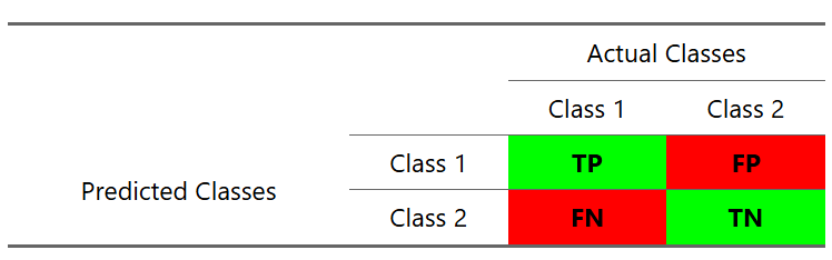
At first, the terminology can be confusing. A simple way to interpret it is that positive and negative refer to the predicted class (whether we predict the event or not), while true and false refer to whether the prediction is correct. For instance, in a medical test for a virus, a positive prediction means we predict that the virus is present. If the person actually has the virus, this is a true positive (correct prediction). If the person does not have the virus, it becomes a false positive.
Confusion Matrix Layout Conventions
The layout of the confusion matrix is not fixed. In some sources, the actual values are placed in rows and predictions in columns, while in others the opposite is used. This is purely a matter of convention; the interpretation of TP, TN, FP, and FN remains the same.
A confusion matrix allows us to compute several performance metrics. The simplest is accuracy, which we have already used in previous chapters. As discussed in Chapter K-Nearest Neighbors, accuracy is defined as the proportion of correct predictions:
\[\text{Accuracy} = \frac{\text{Number of correct predictions}}{\text{Number of observations}}\]
Using the confusion matrix notation, accuracy can also be written in the following way:
\[\text{Accuracy} = \frac{\text{TP} + \text{TN}}{\text{TP} + \text{TN} + \text{FP} + \text{FN}}\]
The interpretation is straightforward: we measure the proportion of correct predictions among all predictions. However, accuracy treats all classes equally and does not account for class imbalance. For example, if one class represents 80% of the data, a naive model that always predicts this majority class will already achieve 80% accuracy without any real predictive power.
An alternative metric is Cohen’s Kappa (Cohen, 1960; Agresti, 2012; Kuhn et al., 2019). This metric adjusts accuracy by taking into account the agreement that would be expected by chance. In other words, it compares the observed accuracy with the accuracy we would expect if predictions were made randomly according to class proportions. As a result, Kappa provides a more conservative evaluation when class imbalance is present.
Mathematically, Cohen’s Kappa is defined as:
\[\kappa = \frac{p_o - p_e}{1 - p_e}\]
where \(p_o\) is the observed accuracy (i.e., the proportion of correct predictions), and \(p_e\) is the expected accuracy under random chance agreement. The value of \(p_e\) is computed based on the marginal proportions of the confusion matrix. Intuitively, it represents how often we would expect the model and the true labels to agree purely by chance if both were generating labels independently but following the same class distribution.
To interpret Kappa, we compare the improvement over chance relative to the maximum possible improvement. A value of \(\kappa = 1\) indicates perfect agreement between predictions and actual values, while \(\kappa = 0\) indicates that the model performs no better than random guessing. Kappa can also take negative values, suggesting a performance worse than random guessing.
Intuitively, while accuracy rewards any correct prediction equally, Cohen’s Kappa asks a more strict question: “How much better is this model compared to simply guessing based on class frequencies?” This makes it especially useful when one class dominates the dataset, since a naive model can achieve high accuracy without learning meaningful patterns.
A third important metric is the Matthews Correlation Coefficient (MCC). MCC measures the correlation between the observed and predicted classifications and takes into account all four elements of the confusion matrix (TP, TN, FP, FN). Unlike accuracy and Kappa, MCC is particularly robust in the presence of class imbalance because it considers both types of errors in a balanced way. For this reason, MCC is often preferred when the dataset is highly imbalanced (Lantz, 2023).
Interestingly, if we encode the classes as 1 and 0 and compute the Pearson correlation coefficient between the true and predicted values, we obtain exactly the same result as MCC (Lantz, 2023). In this sense, MCC can be interpreted as a correlation-based measure of classification quality, capturing how strongly predictions align with the actual classes in a single value that ranges from -1 (total disagreement) to 1 (perfect agreement).
All these metrics focus on the overall performance of a classifier, combining TP and TN results in the same way. However, in many applications we are interested in distinguishing between different types of errors. Sensitivity and specificity are two metrics that focus on this distinction.
Sensitivity measures how well the model identifies the event of interest (the positive class). It is defined as:
\[\text{Sensitivity} = \frac{\text{TP}}{\text{TP} + \text{FN}}\]
Sensitivity can be interpreted as the proportion of actual positives that are correctly identified by the model. In other words, it answers the question: “Out of all real events, how many did we detect?” On the confusion matrix, this corresponds to the proportion of the positive class row that is correctly classified as TP. A perfect model would have no false negatives, meaning that all actual events are correctly detected. At the extreme, a naive model that always predicts the event would achieve perfect sensitivity, since it would never miss a positive case.
Specificity is the mirror image of specificity. It measures how well the model identifies the non-event (the negative class). It is defined as:
\[\text{Specificity} = \frac{\text{TN}}{\text{TN} + \text{FP}}\]
Specificity represents the proportion of actual negatives that are correctly classified. Intuitively, it answers: “Out of all non-events, how many did we correctly rule out?” On the confusion matrix, this corresponds to the proportion of the negative class row that is correctly classified as TN.
Together, sensitivity and specificity provide a more detailed view of model performance than accuracy alone, since they separate the ability to detect positives from the ability to correctly reject negatives.
However, in many classification problems we are primarily interested in correctly identifying the positive class (the event of interest). In these cases, we focus on metrics based on positive predictions, namely precision and recall.
Precision measures how many of the predicted positives are actually correct:
\[\text{Precision} = \frac{\text{TP}}{\text{TP} + \text{FP}}\]
It answers the question: “When the model predicts an event, how often is it correct?”. More precisely, precision focuses on the reliability of positive predictions, penalizing false alarms (FP). A high precision means that when the model predicts the event, it is usually correct.
Recall measures how many of the true positives are actually captured by the model:
\[\text{Recall} = \frac{\text{TP}}{\text{TP} + \text{FN}}\]
This formula is actually the same as sensitivity, meaning both terms are used interchangeably. The difference is mostly contextual: “recall” is more common in machine learning, while “sensitivity” is often used in statistics and medical settings.
There is typically a trade-off between precision and recall. If we make the model more “strict” about predicting positives, we reduce false positives and increase precision, but we may miss more actual positives, lowering recall. Conversely, if we make the model more “permissive” about predicting positives, we increase recall but may introduce more false positives, reducing precision.
An example that illustrates this trade-off is airplane safety classification. Suppose we have a model that predicts whether a plane is safe to depart, where a “positive” prediction represents a crash risk. On one extreme, we could predict that every plane is unsafe (all positive predictions). In this case, recall would be perfect, because we would correctly identify all planes that would actually crash. In this case, there would be no false negatives—no planes that would actually crash would be incorrectly predicted as safe. However, precision would be extremely low, since most of our “unsafe” predictions would be false alarms—the high number of false positives would inflate the denominator in the precision formula. On the other extreme, we could predict that almost all planes are safe to fly. In this case, precision would be high, since we would only rarely predict a crash risk, and most of those predictions would (probably) be correct. However, recall would be low, as we would fail to detect the majority of actual crash cases. Note that if we predict every flight as safe (i.e., make only negative predictions), both metrics would be 0, since we would never predict a positive event, resulting in zero true positives as well as zero false positives.
This example illustrates the trade-off between precision and recall. The acceptable trade-off between these two metrics depends on the application. For instance, in medical screening we may prioritize recall, while in spam detection we may prioritize precision. A metric that combines both precision and recall is the F-measure (or F1-score). This metric uses the harmonic mean, meaning it penalizes extreme imbalance between the two metrics and only gives a high value when both are high.
The F1-score ranges between 0 and 1, where 0 indicates the worst possible performance and 1 indicates perfect precision and recall. The mathematical formula is the following:
\[\text{F1-score} = \frac{2 \times \text{precision} \times \text{recall}}{\text{precision} + \text{recall}} = \frac{2 \times \text{TP}}{2 \times \text{TP} + \text{FP} + \text{FN}}\]
In this formula, the harmonic mean ensures that the F-score will only be high if both precision and recall are high. This happens because the metric is not a simple average, but a ratio that depends on both values simultaneously.
To see this more clearly, rewrite the F1-score as:
\[\text{F1-score} = \frac{2}{\frac{1}{\text{precision}} + \frac{1}{\text{recall}}}\]
From this form, it becomes clear that if either precision or recall is small, its reciprocal becomes large, which increases the denominator and reduces the overall score. As a result, even if one metric is very high, the F-score will still be pulled down by the low value of the other. In other words, the harmonic mean penalizes imbalance: it does not allow one metric to compensate for the other. This is why the F-score only becomes large when both precision and recall are simultaneously high.
Finally, it is important to note that the F1-score is a default choice that gives equal weight to precision and recall. In practice, this balance can be adjusted depending on the problem at hand by tuning the weight parameter (\(\beta\)). Therefore, the more general form of the F-score is given by:
\[F_\beta = \frac{(1 + \beta ^ 2) \times \text{precision} \times \text{recall}}{\beta ^ 2 \times \text{precision} + \text{recall}}\]
where \(\beta\) controls the relative importance of recall compared to precision. More specifically, values of \(\beta > 1\) place more emphasis on recall, while values of \(\beta < 1\) place more emphasis on precision. In this formula, it is apparent that when \(\beta = 1\), then \(F_\beta = F_1\).
Metrics for Soft Classification Tasks
Apart from hard classification, where predictions are assigned directly to a class, we can also use soft classification. In this case, instead of predicting a class label, the model outputs probabilities for each class. For example, rather than predicting that a customer will churn, the model may output a probability of 0.8 for churn and 0.2 for no churn. These probabilities allow us to make more flexible decisions, depending on how strict we want the classification to be.
All hard classification metrics provide a single number to evaluate performance, based on a fixed threshold (usually 0.5) that converts probabilities into class labels. However, this choice of threshold is arbitrary and may not be optimal for every application. For this reason, it is often useful to evaluate model performance across all possible thresholds, rather than relying on a single one.
The Receiver Operating Characteristic (ROC) curve is a graphical tool that illustrates the trade-off between the True Positive Rate (sensitivity) and the False Positive Rate (1 − specificity) across different classification thresholds. Instead of fixing a single cutoff value, we vary the threshold from 0 to 1 and compute the corresponding sensitivity and false positive rate at each step.
Historically, ROC curves originate from signal detection theory and were first developed during World War II to evaluate radar systems, where the goal was to distinguish between true signals (e.g., enemy aircraft) and noise. This idea was later adopted in statistics and machine learning as a way to evaluate classification models (Swets, 1988).
The following code illustrates how we can compute and visualize the ROC curve using scikit-learn. Since this section is purely illustrative, we generate a small synthetic two-class dataset rather than relying on a specific real-world example:
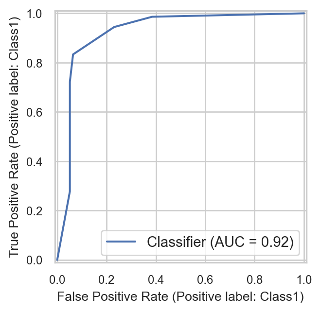
The plot shows the False Positive Rate (1 - specificity) on the x-axis and the True Positive Rate (sensitivity) on the y-axis. Each point on the curve corresponds to a different classification threshold. A model with no predictive power would produce a diagonal line, indicating that it performs no better than random guessing. In contrast, a good model will produce a curve that bends toward the top-left corner, indicating high sensitivity and low false positive rate.
In contrast to hard classification metrics, the ROC curve is less sensitive to class imbalance. This is because it focuses on rates (proportions) rather than absolute counts, making it more robust when one class is much more frequent than the other.
To summarize the ROC curve into a single number, we use the Area Under the Curve (AUC). The AUC measures the overall ability of the model to distinguish between the two classes across all possible classification thresholds. In other words, it evaluates how well the model separates positive and negative observations based on their predicted scores, rather than relying on a single cutoff value. The AUC takes values between 0 and 1:
\(0 < \text{AUC} \le 0.5\): the model performs worse than or equal to random guessing. A value close to 0.5 (e.g., 0.45) indicates random-like performance, meaning the model has no meaningful ability to distinguish between the two classes. Values below 0.5 suggest that the model is systematically ranking negative cases higher than positive ones, which can often be interpreted as an inverted model 0.5.
\(0.5 < \text{AUC} \le 1\) : the model performs better than random guessing, with higher values indicating stronger discrimination ability. An AUC of 1 represents perfect classification, meaning that all positive observations receive higher predicted scores than all negative observations.
An intuitive interpretation of AUC is that it represents the probability that the model assigns a higher predicted probability to a randomly chosen positive observation than to a randomly chosen negative observation. Thus, higher AUC values indicate better ranking ability of the model, which is particularly useful when the goal is to prioritize or rank cases rather than make hard classification decisions. For example, if we take one patient who actually has a disease and one who does not, AUC measures how often the model assigns a higher disease probability to the sick patient than to the healthy one.
In practice, ROC-AUC is widely used because it provides a threshold-independent measure of performance. However, it should be interpreted together with other metrics, especially when the application requires prioritizing either false positives or false negatives. In this sense, ROC-AUC can be seen as the soft classification counterpart of sensitivity and specificity, since it evaluates their trade-off across all possible thresholds rather than at a single cutoff point. Instead of fixing a threshold and computing one pair of sensitivity and specificity values, ROC analysis summarizes how these two quantities evolve together as the threshold changes.
A similar idea can be applied to precision and recall. Instead of evaluating them at a single threshold, we can construct a precision–recall (PR) curve, which illustrates the trade-off between these two metrics across different thresholds. Just like the ROC curve, each point on the PR curve corresponds to a different classification threshold.
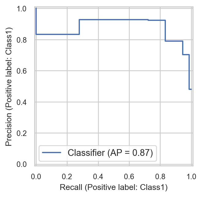
The interpretation is also similar: as we move along the curve, increasing recall typically leads to a decrease in precision, and vice versa. This reflects the same trade-off we discussed earlier, but now evaluated across all possible decision thresholds rather than at a fixed one.
In practice, the precision–recall curve is particularly useful when dealing with imbalanced datasets. While ROC curves can sometimes present an overly optimistic view in such cases, PR curves focus directly on the performance of the positive class, making them more informative when the event of interest is rare.
As with ROC-AUC, we can summarize the precision–recall curve into a single number, often referred to as the area under the precision–recall curve. This provides an overall measure of how well the model balances precision and recall across different thresholds, complementing the insights obtained from ROC-AUC.
Performance Metrics with Scikit-learn
The regression and classification metrics are often harder to understand and choose appropriately than they are to implement. Especially with scikit-learn, the implementation of these metrics is fairly straightforward, since they’re all available as ready-to-use functions in sklearn.metrics.
The functions for the metrics discussed throughout this chapter are the following:
mean_absolute_error(): Mean absolute error (MAE)mean_squared_error()(withsquared = False, or wrapped innp.sqrt()): Root mean squared error (RMSE)r2_score(): R-squaredconfusion_matrix(): Confusion matrixaccuracy_score(): Overall accuracycohen_kappa_score(): Cohen’s Kappamatthews_corrcoef(): Matthews Correlation Coefficientrecall_score()(computed on the positive class): Sensitivityrecall_score()(computed on the negative class): Specificityprecision_score(): Precisionrecall_score(): Recallf1_score(): F-measure (F1-score by default)roc_auc_score(): ROC-AUC
All these functions require the actual values and the predicted values as separate arguments. Typically, we pass the true labels first, followed by the predicted class labels. The function roc_auc_score(), however, does not take predicted class labels; instead, it requires the predicted probabilities for the positive class.
To illustrate how these metrics can be used, we reuse the predictions from the synthetic two-class example introduced in the previous section, and organize them into a DataFrame with the structure truth, Class1, Class2, and predicted:
# Building a dataframe with truth, predicted probabilities, and predicted labels
two_class_example = pd.DataFrame({
  "truth": y_test_clf,
  "Class1": pred_probs,
  "Class2": 1 - pred_probs,
  "predicted": model.predict(X_test_clf)
  })

# Printing the first few rows
two_class_example.head()| truth | Class1 | Class2 | predicted | |
|---|---|---|---|---|
| 0 | Class1 | 0.94 | 0.06 | Class1 |
| 1 | Class2 | 1.00 | 0.00 | Class1 |
| 2 | Class1 | 0.94 | 0.06 | Class1 |
| 3 | Class1 | 1.00 | 0.00 | Class1 |
| 4 | Class1 | 0.94 | 0.06 | Class1 |
The two_class_example DataFrame has four columns:
truth: the actual class labelsClass1: predicted probabilities for Class 1Class2: predicted probabilities for Class 2predicted: predicted class labels
The following code shows how we can create a confusion matrix and calculate all classification metrics:
from sklearn.metrics import (
    confusion_matrix, accuracy_score, cohen_kappa_score, matthews_corrcoef,
    recall_score, precision_score, f1_score, roc_auc_score
)

# Confusion matrix
confusion_matrix(two_class_example["truth"],
                 two_class_example["predicted"],
                 labels = ["Class1", "Class2"])
array([[68, 4],
[18, 60]])# Accuracy
accuracy_score(two_class_example["truth"],
two_class_example["predicted"])0.8533333333333334# Cohen's Kappa
cohen_kappa_score(two_class_example["truth"],
two_class_example["predicted"])0.7083775185577943# Matthews Correlation Coefficient
matthews_corrcoef(two_class_example["truth"],
two_class_example["predicted"])0.7208998757722819# Sensitivity
recall_score(two_class_example["truth"],
two_class_example["predicted"],
pos_label = "Class1")0.9444444444444444# Specificity
recall_score(two_class_example["truth"],
two_class_example["predicted"],
pos_label = "Class2")0.7692307692307693# Precision
precision_score(two_class_example["truth"],
two_class_example["predicted"],
pos_label = "Class1")0.7906976744186046# Recall
recall_score(two_class_example["truth"],
two_class_example["predicted"],
pos_label = "Class1")0.9444444444444444# F1-score
f1_score(two_class_example["truth"],
two_class_example["predicted"],
pos_label = "Class1")0.8607594936708861# ROC-AUC score
roc_auc_score((two_class_example["truth"] == "Class1").astype(int), two_class_example["Class1"])0.92485754985755Regarding resampling, we can actually compute multiple metrics at once using cross_validate(), the same function we used for k-fold cross-validation earlier—we just pass a list of metric names to scoring instead of a single one. To illustrate, let’s calculate MAE, RMSE, and R-squared together using our repeated k-fold splits, splits_rep_cv:
# Fitting resamples to calculate MAE, RMSE and R-squared
results_rep_cv_multi = cross_validate(
  lm_workflow,
  X_train,
  y_train,
  cv = splits_rep_cv,
  scoring = ["neg_mean_absolute_error", "neg_root_mean_squared_error", "r2"]
  )

# Flipping the sign on the error metrics to get them back on their normal scale
mae = -results_rep_cv_multi["test_neg_mean_absolute_error"]
rmse = -results_rep_cv_multi["test_neg_root_mean_squared_error"]
rsq = results_rep_cv_multi["test_r2"]

# Collecting results
pd.DataFrame({
  "metric": ["mae", "rmse", "rsq"],
  "mean": [mae.mean(), rmse.mean(), rsq.mean()],
  "std_err": [mae.std(ddof = 1) / np.sqrt(len(mae)),
              rmse.std(ddof = 1) / np.sqrt(len(rmse)),
              rsq.std(ddof = 1) / np.sqrt(len(rsq))]
})| metric | mean | std_err | |
|---|---|---|---|
| 0 | mae | 5341.89 | 295.75 |
| 1 | rmse | 6704.29 | 417.42 |
| 2 | rsq | 0.55 | 0.06 |
Unlike MAE and RMSE, a higher R-squared is already better, so scikit-learn doesn’t need to flip its sign.
The output now consists of multiple rows, one for each metric. For each metric, we obtain the average performance across all resamples, along with measures such as the standard error. This allows us to evaluate the model from different perspectives—for example, comparing absolute errors (MAE), penalizing large errors (RMSE), and assessing explained variance (R-squared)—all within a single, consistent framework. In practice, this flexibility is particularly useful, as different metrics may highlight different strengths and weaknesses of the same model.
Recap
In this chapter, we focused on resampling methods such as k-fold cross-validation, Monte Carlo cross-validation, and bootstrap. These methods allow us to evaluate models multiple times on different splits of the data, providing a more stable and robust estimate of performance than a single train–test split. We also highlighted how different resampling strategies reflect different assumptions about the data, including independence, randomness, and temporal structure. Additionally, we showed how these evaluation strategies connect naturally to performance metrics for both regression and classification problems.
Using scikit-learn, we demonstrated how both resampling methods and performance metrics can be implemented within a consistent, reusable set of helper functions, highlighting how the same workflow extends naturally across different resampling strategies and evaluation metrics.